5 Risk-Adjusted Return Formulas for Options Traders

Most traders focus on returns, but not all returns are equal when factoring in risk. Risk-adjusted metrics help you evaluate if the profits you’re making are worth the risks you’re taking. For options traders, where leverage and volatility play a big role, these formulas are essential. Here’s a quick rundown of five key metrics:

Sharpe Ratio: Measures total return against total volatility. Good for comparing strategies but penalizes both upside and downside volatility equally.
Sortino Ratio: Focuses only on downside risk, giving a clearer view of strategies with uneven returns like short puts or covered calls.
Treynor Ratio: Evaluates returns relative to market risk (beta). Best for strategies tied to overall market movements.
Jensen’s Alpha: Shows how much a strategy outperforms its risk-adjusted benchmark. Useful for assessing trading edge.
Capital-at-Risk Efficiency: Examines premium collected relative to capital at risk, highlighting how efficiently your capital is being used.

Each formula has its strengths and blind spots, so combining them offers a more balanced view of your strategy’s risk and reward profile.

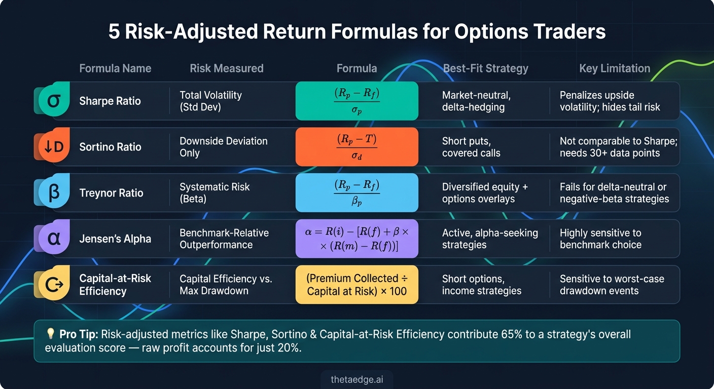
5 Risk-Adjusted Return Formulas for Options Traders Compared

1. Sharpe Ratio for Total Volatility Risk

The Sharpe Ratio is a go-to metric for gauging risk-adjusted performance. Its formula is simple: (Rp – Rf) / σp, where Rp represents your portfolio's return, Rf is the risk-free rate (often the 3-month U.S. Treasury bill yield, which was in the 3.8%–4.1% range as of April 2026), and σp is the standard deviation of your returns. Essentially, it measures how much excess return you're earning for each unit of volatility.

For options traders, this ratio makes comparing strategies straightforward. Take a vertical spread with an 18% return and a 10% standard deviation - that gives a Sharpe Ratio of 1.4. Now compare it to an iron condor delivering a 12% return with only a 6% standard deviation. Its Sharpe Ratio comes out to 1.33. While the vertical spread offers a higher raw return, the iron condor is nearly as efficient when adjusted for risk. This ability to distill performance into one clear number is where the Sharpe Ratio shines.

Covered call strategies, for instance, can elevate Sharpe Ratios by 36% to 73% compared to simply holding index funds. They achieve this by cutting portfolio volatility by 30%–40%, while only giving up 0.5%–1.5% in annual returns. Meanwhile, short puts provide steady premium income and improve Sharpe Ratios during stable markets. However, they come with tail risks that standard deviation doesn’t fully capture. This gap underscores the need for other metrics to complement the Sharpe Ratio when evaluating options strategies.

"A strategy can have low volatility and catastrophic tail risk (selling out-of-the-money options, picking up nickels in front of a steamroller). Sharpe will flatter that strategy until the tail event arrives." - Ferrante Advisors

One limitation of the Sharpe Ratio is that it treats all volatility the same, penalizing gains just as much as losses. For options sellers, this can paint an overly optimistic picture. Moreover, the ratio assumes returns follow a normal distribution, but options strategies often result in skewed, fat-tailed outcomes that break this assumption. While it’s a great starting point, the Sharpe Ratio isn’t the whole story. Traders should pair it with other tools to fully understand the risks and rewards of their strategies.

2. Sortino Ratio for Downside Risk Only

The Sortino Ratio refines the Sharpe Ratio by narrowing its focus to downside risk, offering a clearer picture of risk-adjusted returns. Unlike the Sharpe Ratio, which penalizes both upward and downward volatility, the Sortino Ratio only considers the downside. Its formula is (Rp – T) / σd, where Rp represents your portfolio return, T is the benchmark return (often 0% or the risk-free rate), and σd is the downside deviation - the standard deviation of returns that fall below your target. Positive returns above the target are ignored, ensuring they don’t negatively impact the calculation.

"Upside volatility is desirable, and penalizing a strategy for excess gains is illogical." - StratBase.ai

This approach is particularly relevant for options traders. For instance, strategies like short puts or covered calls often generate consistent small profits with occasional sharp losses. The Sharpe Ratio might penalize these strategies for large winning months by treating them as volatility, while the Sortino Ratio focuses exclusively on downside risk. This distinction often results in the Sortino Ratio being 1.3x to 1.7x higher than the Sharpe Ratio for the same strategy. By concentrating on downside performance, the Sortino Ratio provides a more precise evaluation for strategies where gains and losses behave asymmetrically.

To calculate the Sortino Ratio, you’ll need historical returns, a defined Minimum Acceptable Return (MAR, typically 0%), and the downside deviation (calculated only from returns below the MAR). It’s important to note that fewer than 30 trades or 24–36 monthly observations can lead to unreliable results.

However, the Sortino Ratio has its own limitations. It does not account for tail risk, meaning strategies like put-selling may show a strong ratio until a sudden market shock wipes out gains. Similarly, long-volatility strategies can appear less favorable due to steady theta decay, even when performing as expected.

Sortino Ratio	What It Signals
Below 0.0	Strategy is losing money relative to the target
0.5 – 1.0	Acceptable, but not impressive
1.0 – 2.0	Good; reflects solid compensation for downside risk
2.0 – 3.0	Strong; indicates high returns relative to downside volatility
Above 3.0	Exceptional - but may require scrutiny for potential data issues or over-fitting

3. Treynor Ratio for Market Beta Risk

While the Sortino Ratio focuses on downside volatility, the Treynor Ratio measures how much excess return you’re earning per unit of market risk. The formula is straightforward: (Rp – Rf) / βp. Here, Rp represents your portfolio return, Rf is the risk-free rate (often the 3-month U.S. Treasury yield), and βp is your portfolio's beta, which reflects its sensitivity to market movements like those of the S&P 500. This makes the Treynor Ratio particularly useful for strategies that are heavily influenced by market beta.

For options traders with directional positions, your position's delta plays a role in determining its overall market beta. The Treynor Ratio helps assess whether the returns or premiums you generate are sufficient to justify the market risk you’ve taken on.

"The Treynor ratio captures exactly this: it rewards managers for returns earned per unit of market exposure, without penalizing them for diversifiable risk that no longer exists in the portfolio." - Ryan O'Connell, CFA, FRM

To calculate the Treynor Ratio effectively, you need three inputs measured over the same period: your realized or expected return, the risk-free rate, and an estimate of beta. Beta calculations are typically based on 36 to 60 months of historical data to ensure stability. A Treynor Ratio higher than the market’s own excess return (Rm – Rf) indicates that your portfolio is outperforming on a risk-adjusted basis, given the level of systematic risk.

However, the Treynor Ratio has its limitations for options traders. Unlike the Sharpe and Sortino Ratios, which account for total and downside volatility, the Treynor Ratio focuses solely on market exposure. This assumes a linear relationship between risk and return, which doesn’t align with the non-linear nature of options' Greeks. For strategies like delta-neutral or hedging, the ratio becomes problematic. A near-zero beta renders the ratio undefined, while a negative beta - common with protective puts - can flip the result, potentially leading to confusion. Additionally, metrics like gamma and vega introduce complexities that beta alone cannot address. As such, the Treynor Ratio is better suited for diversified, directionally exposed portfolios rather than individual options positions.

Here’s a quick breakdown of how different scenarios impact the Treynor Ratio:

Scenario	Beta (βp)	Excess Return	Treynor Result
Strong directional strategy	Positive	High positive	High - efficient use of market risk
Underperforming directional strategy	Positive	Low positive	Low - less efficient than the market
Protective put / negative beta	Negative	Positive	Negative - potentially misleading
Delta-neutral strategy	Near zero	Any	Undefined - ratio loses interpretive value

4. Jensen's Alpha for Risk-Adjusted Outperformance

Jensen's Alpha evaluates how much extra return a portfolio generates beyond what the CAPM (Capital Asset Pricing Model) predicts, given the level of market risk taken. The formula is: α = R(i) – [R(f) + β × (R(m) – R(f))].

In simple terms, you compare your portfolio's actual return to the return CAPM expects based on its beta (market sensitivity). A positive alpha indicates outperformance due to factors like timing, strike selection, or portfolio structure. A negative alpha means the portfolio underperformed relative to the risk taken, while zero suggests performance aligned perfectly with CAPM predictions.

To calculate Jensen's Alpha, you’ll need four key inputs, all measured over the same time frame:

Portfolio's realized return (R(i))
Benchmark return (R(m)): Often the S&P 500, though a Nasdaq-specific index might be more suitable for certain options strategies. Using an inappropriate benchmark can skew your alpha calculation.
Risk-free rate (R(f))
Portfolio beta (β)

Let’s break it down with an example. Assume your covered call portfolio achieved a 15% return during a period when the S&P 500 returned 12%, the 3-month Treasury bill rate was 3%, and your portfolio beta was 1.2. Using the CAPM formula:

CAPM-predicted return = 3% + 1.2 × (12% – 3%) = 13.8%

Jensen's Alpha = 15% – 13.8% = +1.2%

This result shows your portfolio outperformed on a risk-adjusted basis by 1.2%. However, this calculation doesn’t account for the unique characteristics of options trading.

Options bring complexities that Jensen’s Alpha doesn’t fully capture. For example, options have convexity (Gamma), are influenced by time decay (Theta), and are sensitive to changes in implied volatility (Vega). Beta, as used in CAPM, doesn’t reflect these factors. As Alpha Learning puts it:

"A single option position embeds exposure to price moves, time, and volatility. Traders who only think about directional bias miss dominant drivers like time decay or implied volatility shifts." - Alpha Learning

Because of these limitations, Jensen's Alpha is best viewed as a benchmark for comparing performance rather than a comprehensive risk measure. It works well when paired with tools like the Sharpe and Sortino Ratios, which provide insights into total and downside volatility. Always keep an eye on your options Greeks to account for the nuances of options trading.

5. Capital-at-Risk Efficiency Ratio for Options Exposure

The Capital-at-Risk Efficiency Ratio, often referred to as Return on Capital (ROC), is a key metric for options traders. It measures the premium collected relative to the capital you’re risking. The formula is simple: Efficiency Ratio = (Premium Collected ÷ Capital at Risk) × 100.

What makes this ratio so practical is its ability to compare performance across different trade structures. For example, consider a cash-secured put on a $100 stock at a $95 strike. This trade might generate $3.50 in premium but requires about $9,150 in capital, giving it a raw ROC of approximately 3.8%. On the other hand, a $5-wide put credit spread on the same strike might collect $1.50 in premium but only risks $350, resulting in a ROC of around 42.9%. Both trades involve the same stock and directional bias, but the capital efficiency is vastly different.

"ROC tells you how hard your capital is working. Compare ROC across different setups on the same stock to find the most efficient trade." - Aigars Pilmanis, VolRadar

Most premium sellers aim for a per-trade ROC between 20% and 40% before annualizing. However, after factoring in costs, slippage, and taxes, long-term annualized figures typically range from 10% to 25%. Chasing extremely high efficiency ratios, such as those exceeding 60%, can be risky. Such numbers often indicate either extreme implied volatility or a very low Probability of Profit (POP). As Pomegra's Learn Library cautions: "High capital efficiency is useless if it comes with 50% account drawdowns. Sustainable efficiency pairs lower drawdown with consistent returns."

It’s also crucial to use accurate inputs for this calculation. Annualizing ROC assumes continuous capital redeployment, which doesn’t account for idle periods, drawdowns, or compounding risks. Additionally, you should consult your broker for the Buying Power Reduction (BPR). Different platforms calculate BPR differently - some subtract the credit received from the margin requirement, while others hold the full spread width. These differences can significantly affect your efficiency calculations.

For traders looking to streamline these comparisons, tools like ThetaEdge provide pre-analyzed, risk-adjusted data for various options strategies, making it easier to evaluate capital efficiency across setups.

Comparison Table

Each formula addresses a specific type of risk, making them uniquely suited to different strategies. The table below provides a concise overview of their focus, ideal use cases, data needs, and potential limitations:

Formula	Risk Measured	Best-Fit Options Strategy	Data Requirements	Limitation
Sharpe Ratio	Total volatility (standard deviation)	Market-neutral, delta-hedging	Return, risk-free rate, standard deviation	Penalizes upside volatility; conceals tail risk in short-volatility strategies
Sortino Ratio	Downside deviation only	Long options, trend-following	Return, target return, downside deviation	Not directly comparable to Sharpe; sensitive to sample size
Treynor Ratio	Systematic risk (Beta)	Diversified equity with options overlays	Return, risk-free rate, Beta	Ignores idiosyncratic (stock-specific) risk
Jensen's Alpha	Benchmark-relative outperformance	Active, alpha-seeking strategies	Return, risk-free rate, Beta, benchmark return	Highly sensitive to benchmark choice
Capital-at-Risk Efficiency	Maximum drawdown	Short options, income strategies	Compound annual growth rate, peak-to-trough maximum drawdown	Highly sensitive to the worst-case event; fluctuates with each new drawdown

This comparison highlights how each metric aligns with specific strategies and risk profiles.

Here are a few practical takeaways:

Sharpe vs. Sortino: The Sharpe Ratio penalizes all types of volatility, including upside gains, which can be a drawback for strategies that benefit from positive swings. In contrast, the Sortino Ratio focuses solely on downside risk and often produces ratios 1.3× to 1.7× higher by ignoring upward volatility gains.
Treynor vs. Jensen's Alpha: Treynor Ratio measures how effectively your strategy uses market exposure (Beta), making it ideal for portfolios that combine options with broader equity positions. Jensen's Alpha, however, digs deeper, showing whether your returns outperform what Beta alone would predict - essentially quantifying your trading edge.

Understanding these distinctions can help you choose the right metric for your specific approach.

Conclusion

Each metric sheds light on a different aspect of a strategy's risk profile, but no single one tells the whole story. Where Sharpe leaves gaps, Sortino steps in; where Treynor and Jensen provide insights, the results depend on factors like market exposure and benchmark choices. Every metric has its blind spots, which is why they’re best used together to paint a fuller picture of risk.

Professionals often combine multiple metrics to achieve a more balanced view of risk. In high-efficiency trading models, risk-adjusted metrics like Sharpe, Sortino, and Capital-at-Risk Efficiency contribute 65% to a strategy's overall evaluation score, while raw profit accounts for just 20%. By using these formulas in tandem, traders gain a more thorough understanding of risk-adjusted returns.

"No single metric captures everything. The industry uses multiple metrics together. Combining metrics into a Weighted Risk Score helps balance multiple dimensions and prevents being fooled by one shiny number." - Philipp Tschakert

This highlights the value of taking a diversified approach to risk assessment.

The real challenge lies in applying these formulas to your actual positions, and that's where ThetaEdge steps in. The platform offers Portfolio Greeks, probability metrics, and risk/reward analysis tailored to your specific holdings, whether you're trading covered calls, cash-secured puts, or multi-leg strategies. Instead of relying on generic examples, you can use these tools to analyze the positions you truly hold.

The metrics discussed here are just tools, but when combined and backed by real portfolio data, they turn decision-making into a structured, evidence-based process rather than relying on gut instinct.

FAQs

Which metric fits my options strategy best?

Choosing the right metric comes down to what aligns with your goals and how much risk you're comfortable taking. For many options traders, the Sortino Ratio stands out because it zeroes in on downside risk, unlike the Sharpe Ratio, which treats upside volatility as a negative. If you're comparing strategies, look at the Alpha metric - calculated as Expected Value ÷ Max Loss - to gauge performance. For assessing long-term resilience, focus on Premium Yield on Risked Capital (PYR) and Effective Cost Basis, as these tie your results to intrinsic value rather than surface-level metrics.

How many trades do I need for reliable ratios?

When calculating expectancy and ratios, it's best to analyze a minimum of 30–50 trades, though reviewing 100 or more trades provides a clearer picture of your strategy's performance. Smaller sample sizes can distort results, often failing to capture the true effectiveness of your approach. While some may use as few as 20 trades for illustrative purposes, this is risky. The standard error in such small samples is too large, potentially including zero, which undermines the reliability of expectancy measurements.

How do I estimate beta for an options portfolio?

To estimate beta for an options portfolio, you can use tools available on most brokerage platforms, which typically calculate beta for you. Beta reflects how a stock's price moves in relation to a benchmark, such as the S&P 500.

When it comes to options, beta-weighted delta is a helpful metric. It standardizes position deltas into a comparable unit using this formula:

Position Delta × Stock Price × Beta / Benchmark Price

By summing these beta-weighted deltas across your portfolio, you can determine its overall market exposure. This insight is crucial for managing directional risks more effectively.

Thetix
Wealth Empowered